Quick Start
When you start fluxus, you will see the welcome text and a prompt – this is called the repl (read evaluate print loop), or console. Generally fluxus scripts are written in text buffers, which can be switched to with ctrl and the numbers keys. Switch to the first one of these by pressing ctrl-1 (ctrl-0 switched you back to the fluxus console).
Now try entering the following command.
(build-cube)
Now press F5 (or ctrl-e) – the script will be executed, and a white cube should appear in the centre of the screen. Use the mouse and to move around the cube, pressing the buttons to get different movement controls.
To animate a cube using audio, try this:
; buffersize and samplerate need to match jack’s
(start-audio “jack-port-to-read-sound-from” 256 44100)

(define (render)
   (colour (vector (gh 1) (gh 2) (gh 3)))
   (draw-cube))

(every-frame (render))
To briefly explain, the (every-frame) function takes a function which is called once per frame by fluxus’s internal engine. In this case it calls a function that sets the current colour using harmonics from the incoming sound with the (gh) - get harmonic function; and draws a cube. Note that this time we use (draw-cube) not (build-cube). The difference will be explained below.
If everything goes as planned, and the audio is connected with some input – the cube will flash in a colourful manner along with the sound.
Now go and have a play with the examples. Load them by pressing ctrl-l or on the commandline, by entering the examples directory and typing fluxus followed by the script filename.
User Guide
When using the fluxus scratchpad, the idea is that you only need the one window to build scripts, or play live. F5 (or ctrl-e) is the key that runs the script when you are ready. Selecting some text (using shift) and pressing F5 will execute the selected text only. This is handy for re-evaluating functions without running the whole script each time.
Camera control
The camera is controlled by moving the mouse and pressing mouse buttons.
- Left mouse button: Rotate
- Middle mouse button: Move
- Right mouse button: Zoom
Workspaces
The script editor allows you to edit 9 scripts simultaneously by using workspaces. To switch workspaces, use ctrl+number key. Only one can be run at once though, hitting f5 will execute the currently active workspace script. Scripts in different workspaces can be saved to different files, press ctrl-s to save or ctrl-d to save-as and enter a new filename (the default filename is temp.scm).
The REPL
If you press ctrl and 0, instead of getting another script workspace, you will be presented with a read evaluate print loop interpreter, or repl for short. This is really just an interactive interpreter similar to the commandline, where you can enter scheme code for immediate evaluation. This code is evaluated in the same interpreter as the other scripts, so you can use the repl to debug or inspect global variables and functions they define. This window is also where error reporting is printed, along with the terminal window you started fluxus from.
One of the important uses of the repl is to get help on fluxus commands. For instance, in order to find out about the build-cube command, try typing:
(help "build-cube")
You can find out about new commands by typing
(help "sections")
Which will print out a list of subsections, so to find out about maths commands you can try:
(help "maths")
Will give you a list of all the maths commands availible, which you can ask for further help about. You can copy the example code by moving the cursor left and then up, shift select the code, press ctrl-c to copy it. Then you can switch to a workspace and paste the example in with ctrl-v order to try running them.
Keyboard commands
ctrl-f : Full screen mode.
ctrl-w : Windowed mode.
ctrl-h : Hide/show the editor.
ctrl-l : Load a new script (navigate with cursors and return).
ctrl-s : Save current script.
ctrl-d : Save as current script (opens a filename dialogue).
ctrl-q : Clear the editor window.
ctrl-b : Blow up cursor.
ctrl-1 to 9 : Switch to selected workspace.
ctrl-0 : Switch to the REPL.
ctrl-p : Auto format the white space in your scheme script to be more pretty and readable
F3 : Resets the camera.
F4 : Execute the current highlighted s-expression
F5/ctrl-e : Execute the selected text, or all if none is selected.
F6 : Reset interpreter, and execute text
F9 : Switch scratchpad effects on/off
F10 : Make the text more transparent
F11 : Make the text less transparent
Scheme
Scheme is a programming language invented by Gerald J. Sussman and Guy L. Steel Jr. in 1975. Scheme is based on another language – Lisp, which dates back to the fifties. It is a high level language, which means it is biased towards human, rather than machine understanding. The fluxus scratchpad embeds a Scheme interpreter (it can run Scheme programs) and the fluxus modules extend the Scheme language with commands for 3D computer graphics.
This chapter gives a very basic introduction to Scheme programming, and a fast path to working with fluxus – enough to get you started without prior programming experience, but I don’t explain the details very well. For general scheme learning, I heartily recommend the following books (two of which have the complete text on-line):
The Little Schemer Daniel P. Friedman and Matthias Felleisen
How to Design Programs An Introduction to Computing and Programming Matthias Felleisen Robert Bruce Findler Matthew Flatt Shriram Krishnamurthi Online: http://www.htdp.org/2003-09-26/Book/
Structure and Interpretation of Computer Programs Harold Abelson and Gerald Jay Sussman with Julie Sussman Online: http://mitpress.mit.edu/sicp/full-text/book/book.html
We’ll start by going through some language basics, which are easiest done in the fluxus scratchpad using the console mode – launch fluxus and press ctrl 0 to switch to console mode.
Scheme as calculator
Languages like Scheme are composed of two things – operators (things which do things) and values which operators operate upon. Operators are always specified first in Scheme, so to add 1 and 2, we do the following:
fluxus> (+ 1 2)
3
This looks pretty odd to begin with, and takes some getting used to, but it means the language has less rules and makes things easier later on. It also has some other benefits, in that to add 3 numbers we can simply do:
fluxus> (+ 1 2 3)
6
It is common to “nest” the brackets inside one another, for example:
fluxus> (+ 1 (* 2 3))
7
Naming values
If we want to specify values and give them names we can use the Scheme command “define”:
fluxus> (define size 2)
fluxus> size
2
fluxus> (* size 2)
4
Naming is arguably the most important part of programming, and is the simplest form of what is termed “abstraction” - which means to separate the details (e.g. The value 2) from the meaning – size. This is not important as far as the machine is concerned, but it makes all the difference to you and other people reading code you have written. In this example, we only have to specify the value of size once, after that all uses of it in the code can refer to it by name – making the code much easier to understand and maintain.
Naming procedures
Naming values is very useful, but we can also name operations (or collections of them) to make the code simpler for us:
fluxus> (define (square x) (* x x))
fluxus> (square 10)
100
fluxus> (square 2)
4
Look at this definition carefully, there are several things to take into account. Firstly we can describe the procedure definition in English as: To (define (square of x) (multiply x by itself)) The “x” is called an argument to the procedure, and like the size define above – it’s name doesn’t matter to the machine, so:
fluxus> (define (square apple) (* apple apple))
Will perform exactly the same work. Again, it is important to name these arguments so they actually make some sort of sense, otherwise you end up very confused. Now we are abstracting operations (or behaviour), rather than values, and this can be seen as adding to the vocabulary of the Scheme language with our own words, so we now have a square procedure, we can use it to make other procedures:
fluxus> (define (sum-of-squares x y)
            (+ (square x) (square y)))
fluxus> (sum-of-squares 10 2)
104
The newline and white space tab after the define above is just a text formatting convention, and means that you can visually separate the description and it’s argument from the internals (or body) of the procedure. Scheme doesn’t care about white space in it’s code, again it’s all about making it readable to us.
Making some shapes
Now we know enough to make some shapes with fluxus. To start with, leave the console by pressing ctrl-1 – you can go back at any time by pressing ctrl-0. Fluxus is now in script editing mode. You can write a script, execute it by pressing F5, edit it further, press F5 again... this is the normal way fluxus is used.
Enter this script:
(define (render)
    (draw-cube))

(every-frame (render))
Then press F5, you should see a cube on the screen, drag the mouse around the fluxus window, and you should be able to move the camera – left mouse for rotate, middle for zoom, right for translate.
This script defines a procedure that draws a cube, and calls it every frame – resulting in a static cube.
You can change the colour of the cube like so:
(define (render)
    (colour (vector 0 0.5 1))
    (draw-cube))

(every-frame (render))
The colour command sets the current colour, and takes a single input – a vector. Vectors are used a lot in fluxus to represent positions and directions in 3D space, and colours – which are treated as triplets of red green and blue. So in this case, the cube should turn a light blue colour.
Transforms
Add a scale command to your script:
(define (render)
    (scale (vector 0.5 0.5 0.5))
    (colour (vector 0 0.5 1))
    (draw-cube))

(every-frame (render))
Now your cube should get smaller. This might be difficult to tell, as you don’t have anything to compare it with, so we can add another cube like so:
(define (render)
     (colour (vector 1 0 0))
     (draw-cube)
     (translate (vector 2 0 0))
     (scale (vector 0.5 0.5 0.5))
     (colour (vector 0 0.5 1))
     (draw-cube))
(every-frame (render))
Now you should see two cubes, a red one, then the blue one, moved to one side (by the translate procedure) and scaled to half the size of the red one.
(define (render)
     (colour (vector 1 0 0))
     (draw-cube)
     (translate (vector 2 0 0))
     (scale (vector 0.5 0.5 0.5))
     (rotate (vector 0 45 0))
     (colour (vector 0 0.5 1))
     (draw-cube))

(every-frame (render))
For completeness, I added a rotate procedure, to twist the blue cube 45 degrees.
Recursion
To do more interesting things, we will write a procedure to draw a row of cubes. This is done by recursion, where a procedure can call itself, and keep a record of how many times it’s called itself, and end after so many iterations.
In order to stop calling our self as a procedure, we need to take a decision – we use cond for decisions.
(define (draw-row count)
    (cond
        ((not (zero? count))
             (draw-cube)
             (translate (vector 1.1 0 0))
             (draw-row (- count 1)))))

(every-frame (draw-row 10))
Be careful with the brackets – the fluxus editor should help you by highlighting the region each bracket corresponds to. Run this script and you should see a row of 10 cubes. You can build a lot out of the concepts in this script, so take some time over this bit.
Cond is used to ask questions, and it can ask as many as you like – it checks them in order and does the first one which is true. In the script above, we are only asking one question, (not (zero? Count)) – if this is true, if count is anything other than zero, we will draw a cube, move a bit and then call our self again. Importantly, the next time we call draw-row, we do so with one taken off count. If count is 0, we don’t do anything at all – the procedure exits without doing anything.
So to put it together, draw-row is called with count as 10 by every-frame. We enter the draw-row function, and ask a question – is count 0? No – so carry on, draw a cube, move a bit, call draw-row again with count as 9. Enter draw-row again, is count 0? No, and so on. After a while we call draw-row with count as 0, nothing happens – and all the other functions exit. We have drawn 10 cubes.
Recursion is a very powerful idea, and it’s very well suited to visuals and concepts like self similarity. It is also nice for quickly making very complex graphics with scripts not very much bigger than this one.
Animation
Well, now you’ve got through that part, we can quite quickly take this script and make it move.
(define (draw-row count)
     (cond
         ((not (zero? count))
             (draw-cube)
             (rotate (vector 0 0 (* 45 (sin (time)))))
             (translate (vector 1.1 0 0))
             (draw-row (- count 1)))))

 (every-frame (draw-row 10))
time is a procedure which returns the time in seconds since fluxus started running. Sin converts this into a sine wave, and the multiplication is used to scale it up to rotate in the range of -45 to +45 degrees (as sin only returns values between -1 and +1). Your row of cubes should be bending up and down. Try changing the number of cubes from 10, and the range of movement by changing the 45.
More recursion
To give you something more visually interesting, this script calls itself twice – which results in an animating tree shape.
(define (draw-row count)
     (cond
         ((not (zero? count))
             (translate (vector 2 0 0))
             (draw-cube)
             (rotate (vector (* 10 (sin (time))) 0 0))
             (with-state
                 (rotate (vector 0 25 0))
                 (draw-row (- count 1)))
             (with-state
                 (rotate (vector 0 -25 0))
                 (draw-row (- count 1))))))
 (every-frame (draw-row 10))
For an explanation of with-state, see the next section.
Comments
Comments in scheme are denoted by the ; character:
; this is a comment
Everything after the ; up to the end of the line are ignored by the interpreter.
Using #; you can also comment out expressions in scheme easily, for example:
(with-state
    (colour (vector 1 0 0))
    (draw-torus))
(translate (vector 0 1 0))
#;(with-state
     (colour (vector 0 1 0))
     (draw-torus))
Stops the interpreter from executing the second (with-state) expression, thus stopping it drawing the green torus.
Let
Let is used to store temporary results. An example is needed:
(define (animate)
     (with-state
         (translate (vector (sin (time)) (cos (time)) 0))
         (draw-sphere))
     (with-state
         (translate (vmul (vector (sin (time)) (cos (time)) 0) 3))
         (draw-sphere)))

(every-frame (animate))
This script draws two spheres orbiting the origin of the world. You may notice that there is some calculation which is being carried out twice - the (sin (time)) and the (cos (time)). It would be simpler and faster if we could calculate this once and store it to use again. One way of doing this is as follows:
(define x 0)
(define y 0)

(define (animate)
     (set! x (sin (time)))
     (set! y (cos (time)))
     (with-state
         (translate (vector x y 0))
         (draw-sphere))
     (with-state
         (translate (vmul (vector x y 0) 3))
         (draw-sphere)))

(every-frame (animate))
Which is better - but x and y are globally defined and could be used and changed somewhere else in the code, causing confusion. A better way is by using let:
(define (animate)
     (let ((x (sin (time)))
            (y (cos (time))))
        (with-state
            (translate (vector x y 0))
            (draw-sphere))
        (with-state
            (translate (vmul (vector x y 0) 3))
            (draw-sphere))))

(every-frame (animate))
This specifically restricts the use of x and y to inside the area defined by the outer let brackets. Lets can also be nested inside of each other for when you need to store a value which is dependant on another value, you can use let* to help you out here:
(define (animate)
     (let ((t (* (time) 2)) ; t is set here
           (x (sin t)) ; we can use t here
           (y (cos t))) ; and here

         (with-state
             (translate (vector x y 0))
             (draw-sphere))

         (with-state
             (translate (vmul (vector x y 0) 3))
             (draw-sphere))))

(every-frame (animate))
Lambda
Lambda is a strange name, but it's use is fairly straightforward. Where as normally in order to make a function you need to give it a name, and then use it:
(define (square x) (* x x))
(display (square 10))(newline)
Lambda allows you to specify a function at the point where it's used:
(display ((lambda (x) (* x x)) 10))(newline)
This looks a bit confusing, but all we've done is replace square with (lambda (x) (* x x)). The reason this is useful is that for small specialised functions which won't be needed to be used anywhere else it can become very cumbersome and cluttered to have to define them all, and give them all names.
The State Machine
The state machine is the key to understanding how fluxus works, all it really means is that you can call functions which change the current context which has an effect on subsequent functions. This is a very efficient way of describing things, and is built on top of the OpenGl API, which works in a similar way. For example:
(define (draw)
        (colour (vector 1 0 0))
        (draw-cube)
        (translate (vector 2 0 0)) ; move a bit so we can see the next cube
        (colour (vector 0 1 0))
        (draw-cube))
(every-frame (draw))
Will draw a red cube, then a green cube (in this case, you can think of the (colour) call as changing a pen colour before drawing something). States can also be stacked, for example:
(define (draw)
        (colour (vector 1 0 0))
        (with-state
                (colour (vector 0 1 0))
                (draw-cube))
        (translate (vector 2 0 0))
        (draw-cube))
(every-frame (draw))
Will draw a green, then a red cube. The (with-state) isolates a state and gives it a lifetime, indicated by the brackets (so changes to the state inside are applied to the build-cube inside, but do not affect the build-cube afterwards). Its useful to use the indentation to help you see what is happening.
The Scene Graph
Both examples so far have used what is known as immediate mode, you have one state stack, the top of which is the current context, and everything is drawn once per frame. Fluxus contains a structure known as a scene graph for storing objects and their render states.
Time for another example:
(clear) ; clear the scenegraph
(colour (vector 1 0 0))
(build-cube) ; add a red cube to the scenegraph
(translate (vector 2 0 0))
(colour (vector 0 1 0))
(build-cube) ; add a green cube to the scenegraph
This code does not have to be called by (every-frame), and we use (build-cube) instead of (draw-cube). The build functions create a primitive object, copy the current render state and add the information into the scene graph in a container called a scene node.
The (build-*) functions (there are a lot of them) return object id's, which are just numbers, which enable you to reference the scene node after it’s been created. You can now specify objects like this:
(define myob (build-cube))
The cube will now be persistent in the scene until destroyed with
(destroy myob)
with-state returns the result of it’s last expression, so to make new primitives with state you set up, you can do this:
(define my-object (with-state
                (colour (vector 1 0 0))
                (scale (vector 0.5 0.5 0.5))
                (build-cube)))
If you want to modify a object's render state after it’s been loaded into the scene graph, you can use with-primitive to set the current context to that of the object. This allows you to animate objects you have built, for instance:
; build some cubes
(colour (vector 1 1 1))
(define obj1 (build-cube))
(define obj2 (with-state
                (translate (vector 2 0 0))
                (build-cube))

(define (animate)
        (with-primitive obj1
                (rotate (vector 0 1 0)))

        (with-primitive obj2
                (rotate (vector 0 0 1))))

(every-frame (animate))
A very important fluxus command is (parent) which locks objects to one another, so they follow each other around. You can use (parent) to build up a hierarchy of objects like this:
(define a (build-cube))

(define b (with-state
        (parent a)
        (translate (vector 0 2 0))
        (build-cube)))

(define c (with-state
        (parent b)
        (translate (vector 0 2 0))
        (build-cube)))
Which creates three cubes, all attached to each other in a chain. Transforms for object a will be passed down to b and c, transforms on b will effect c. Destroying a object will in turn destroy all child objects parented to it. You can change the hierarchy by calling (parent) inside a (with-primitive). To remove an object from it's parent you can call:
(with-primitive myprim
         (detach))
Which will fix the transform so the object remains in the same global position.
Note: By default when you create objects they are parented to the root node of the scene (all primitives exist on the scene graph somewhere). The root node is given the id number of 1. So another way of un-parenting an object is by calling (parent 1).
Note on grabbing and pushing
Fluxus also contains less well mannered commands for achieving the same results as with-primitive and with-state. These were used prior to version 0.14, so you may see mention of them in the documentation, or older scripts.
(push) ... (pop)
is the same as:
(with-state ...)
and
(grab myprim) ... (ungrab)
is the same as
(with-primitive myprim ...)
They are less safe than (with-*) as you can push without popping or vice-versa, and shouldn’t be used generally. There are some cases where they are still required though (and the (with-*) commands use them internally, so they won’t be going away).
Input
Quite quickly you are going to want to start using data from outside of fluxus to control your animations. This is really what starts making this stuff interesting, after all.
Sound
The original purpose of fluxus and still perhaps it's best use, was as a sound to light vjing application. In order to do this it needs to take real time values from an incoming sound source. We do this by configuring the sound with:
(start-audio “jack-port-to-read-sound-from” 256 44100)
Running some application to provide sound, or just taking it from the input on your sound card, and then using:
(gh harmonic-number)
To give us floating point values we can plug into parameters to animate them. You can test there is something coming through either with:
(every-frame (begin (display (gh 0)) (newline)))
And see if it prints anything other than 0's or run the bars.scm script in examples, which should display a graphic equaliser. It's also useful to use:
(gain 1)
To control the gain on the incoming signal, which will have a big effect on the scale of the values coming from (gh).
Keyboard
Keyboard control is useful when using fluxus for things like non-livecoding vjing, as it's a nice simple way to control parameters without showing the code on screen. It's also obviously useful for when writing games with fluxus.
(key-pressed key-string)
Returns a #t if the key is currently pressed down, for example:
(every-frame
    (when (key-pressed "x")
        (colour (rndvec))
        (draw-cube)))
Draws a cube with randomly changing colour when the x key is pressed.
(keys-down)
Returns a list of the current keys pressed, which is handy in some situations. For keys which aren't able to be described by strings, there is also:
(key-special-pressed key-code-number)
For instance
(key-special-pressed 101)
Returns #t when the “up” cursor key is pressed. To find out what the mysterious key codes are, you can simply run this script:
(every-frame (begin (display (keys-special-down)) (newline)))
Which will print out the list of special keys currently pressed. Press the key you want and see what the code is. Note: These key codes may be platform specific.
Mouse
You can find out the mouse coordinates with:
(mouse-x)
(mouse-y)
And whether mouse buttons are pressed with:
(mouse-button button-number)
Which will return #t if the button is down.
Select
While we're on the subject of the mouse, one of the best uses for it is selecting primitives, which you can do with:
(select screen-x screen-y size)
Which will render the bit of the screen around the x y coordinate and return the id of the highest primitive in the z buffer. To give a better example:
; click on the donuts!
(clear)

(define (make-donuts n)
    (when (not (zero? n))
        (with-state
            (translate (vmul (srndvec) 5))
            (scale 0.1)
            (build-torus 1 2 12 12))
        (make-donuts (- n 1))))

(make-donuts 10)

(every-frame
    (when (mouse-button 1)
        (let ((s (select (mouse-x) (mouse-y) 2)))
            (when (not (zero? s))
                (with-primitive s
                    (colour (rndvec)))))))
OSC
OSC (Open Sound Control) is a standard protocol for communication between arty programs over a network. Fluxus has (almost) full support for receiving and sending OSC messages.
To get you started, here is an example of a fluxus script which reads OSC messages from a port and uses the first value of a message to set the position of a cube:
(osc-source "6543")
(every-frame
    (with-state
        (when (osc-msg "/zzz")
             (translate (vector 0 0 (osc 0))))
            (draw-cube)))
And this is a pd patch which can be used to control the cube's position.
#N canvas 618 417 286 266 10;
#X obj 58 161 sendOSC;
#X msg 73 135 connect localhost 6543;
#X msg 58 82 send /zzz \$1;
#X floatatom 58 29 5 0 0 0 - - -;
#X obj 58 54 / 100;
#X obj 73 110 loadbang;
#X connect 1 0 0 0;
#X connect 2 0 0 0;
#X connect 3 0 4 0;
#X connect 4 0 2 0;
#X connect 5 0 1 0;
Time
I've decided to include time as a source of input, as you could kind of say it comes from the outside world. It's also a useful way of animating things, and making animation more reliable.
(time)
This returns the time in seconds since the program was started. It returns a float number and is updated once per frame.
(delta)
This command returns the time since the last frame. (delta) is a very important command, as it allows you to make your animation frame rate independent. Consider the following script:
(clear)
(define my-cube (build-cube))
(every-frame
        (with-primitive my-cube
                (rotate (vector 5 0 0))))
This rotates my-cube by one degree each frame. The problem is that it will speed up as the framerate rises, and slow down as it falls. If you run the script on a different computer it will move at a different rate. This used to be a problem when running old computer games - they become unplayable as they run too fast on newer hardware!
The solution is to use (delta):
(clear)
(define my-cube (build-cube))
(every-frame
        (with-primitive my-cube
                (rotate (vector (* 45 (delta)) 0 0))))
The cube will rotate at the same speed everywhere - 45 degrees per second. The normal (time) command is not too useful on it's own - as it returns an ever increasing number, it doesn't mean much for animation. A common way to tame it is pass it through (sin) to get a sine wave:
(clear)
(define my-cube (build-cube))
(every-frame
        (with-primitive my-cube
                (rotate (vector (* 45 (sin (time))) 0 0))))
This is also framerate independent and gives you a value from -1 to 1 to play with. You can also record the time when the script starts to sequence events to happen:
(clear)
(define my-cube (build-cube))
(define start-time (time)) ; record the time now
(every-frame
        ; when the script has been running for 5 seconds...
        (when (> (- (time) start-time) 5)
                (with-primitive my-cube
                        (rotate (vector (* 45 (delta)) 0 0)))))
Material Properties
Now you can create and light some primitives, we can also look more at changing their appearance, other than simply setting their colour.
The surface parameters can be treated exactly like the rest of the local state items like transforms, in that they can either be set using the state stack when building primitives, or set and changed later using (with-primitive).
Line and point drawing modifiers (widths are in pixels):
(wire-colour n)
(line-width n)
(point-width n)
Lighting modifiers:
(specular v)
(ambient v)
(emissive v)
(shinyness n)
Opacity:
(opacity n)
(blend-mode src dest)
The opacity command causes primitives to be semi transparent (along with textures with an alpha component). Alpha transparency brings with it some problems, as it exposes the fact that primitives are drawn in a certain order, which changes the final result where opacity is concerned. This causes flicker and missing bits of objects behind transparent surfaces, and is a common problem in realtime rendering.
The solution is usually either to apply the render hint (hint-ignore-depth) which causes primitives to render the same way every frame regardless of what's in front of them, or (hint-depth-sort) which causes primitives with this hint to be sorted prior to rendering every frame, so they render from the furthest to the closest order. The depth is taken from the origin of the primitive, you can view this with (hint-origin).
Texturing
Texturing is a part of the local material state, but is a complex topic worthy of a chapter in it's own right.
Loading textures
 Getting a texture loaded and applied to a primitive is pretty simple:
(with-state
	(texture (load-texture "test.png"))
	(build-cube))
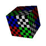
Which applies the standard fluxus test texture to a cube. Fluxus reads png files to use as its textures, and they can be with or without an alpha channel.
The texture loading is memory cached. This means that you can call (load-texture) with the same textures as much as you want, Fluxus will only actually load them from disk the first time. This is great until you change the texture yourself, i.e. if you save over the file from the Gimp and re-run the script, the texture won't change in your scene. To get around this, use:
(clear-texture-cache)
Which will force a reload when (load-texture) is next called on any texture. It's sometimes useful to put this at the top of your script when you are going through the process of changing textures - hitting F5 will cause them to be reloaded.
Texture coordinates
In order to apply a texture to the surface of a primitive, texture coordinates are needed - which tell the renderer what parts of the shape are covered with what parts of the texture. Texture coordinates consist of two values, which range from 0 to 1 as they cross the texture pixels in the x or y direction (by convention these are called "s" and "t" coordinates). What happens when texture coordinates go outside of this range can be changed by you, using (texture-params) but by default the texture is repeated.
The polygon and NURBS shapes fluxus provides you with are all given a default set of coordinates. These coordinates are part of the pdata for the primitive, which are covered in more detail later on. The texture coordinate pdata array is called "t", a simple example which will magnify the texture by a factor of two:
(pdata-map!
	(lambda (t)
		(vmul t 0.5)) ; shrinking the texture coordinates zooms into the texture
	"t")
Texture parameters
There are plenty of extra parameters you can use to change the way a texture is applied.
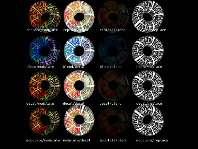
(texture-params texture-unit-number param-list)
We'll cover the texture unit number in multitexturing below, but the param list can look something like this:
(texture-params 0 '(min nearest mag nearest)) ; super aliased & blocky texture :)
The best approach is to have a play and see what these do for yourself, but here are the parameters in full:
tex-env: one of [modulate decal blend replace] 
Changes the way a texture is applied to the colour of the existing surface
min: [nearest linear nearest-mipmap-nearest linear-mipmap-nearest linear-mipmap-linear]
mag: [nearest linear]
These set the filter types which deal with "minification" when the texture's pixels (called texels) are smaller than the screen pixels being rendered to. This defaults to linear-mipmap-linear. Also "magnification", when texels are larger than the screen pixels. This defaults to linear which blends the colour of the texels. Setting this to nearest means you can clearly see the pixels making up the texture when it's large in screen space.
wrap-s: [clamp repeat]
wrap-t: [clamp repeat]
wrap-r: [clamp repeat] (for cube maps)
What to do when texture coordinates are out of the range 0-1, set to repeat by default, clamp "smears" the edge pixels of the texture.
border-colour: (vector of length 4) If the texture is set to have a border (see load-texture) this is the colour it should have.
priority: 0 -> 1
I think this controls how likely a texture is to be removed from the graphics card when memory is low. I've never used this myself though.
env-colour: (vector of length 4)
The base colour to blend the texture with.
min-lod: real number (for mipmap blending - default -1000)
max-lod: real number (for mipmap blending - default 1000)
These set how the mipmapping happens. I haven't had much luck setting this on most graphics cards however.
This is the code which generated the clamp picture above:
(clear)
(texture-params 0 '(wrap-s clamp wrap-t clamp))
(texture (load-texture "refmap.png"))
(with-primitive (build-cube)
    (pdata-map!
        (lambda (t)
            (vadd (vector -0.5 -0.5 0) (vmul t 2)))
    "t"))
Multitexturing
 Fluxus allows you to apply more than one texture to a primitive at once. You can combine textures together and set them to multiply, add or alpha blend together in different ways. This is used in games mainly as a way of using texture memory more efficiently, by separating light maps from diffuse colour maps, or applying detail maps which repeat over the top of lower resolution colour maps.
You have 8 slots to put textures in, and set them with:
(multitexture texture-unit-number texture)
The default texture unit is 0, so:
(multitexture 0 (load-texture "test.png"))
Is exactly the same as
(texture (load-texture "test.png"))
This is a simple multitexturing example:
(clear)
(with-primitive (build-torus 1 2 20 20)
    (multitexture 0 (load-texture "test.png"))
    (multitexture 1 (load-texture "refmap.png")))
By default, all the textures share the "t" pdata as their texture coordinates, but each texture also looks for it's own coordinates to use in preference. These are named "t1", "t2", "t3" and so on up to "t7".
(clear)
(with-primitive (build-torus 1 2 20 20)
    (multitexture 0 (load-texture "test.png"))
    (multitexture 1 (load-texture "refmap.png")))
    (pdata-copy "t" "t1") ; make a copy of the existing texture coords
    (pdata-map!
        (lambda (t1)
            (vmul t1 2)) ; make the refmap.png texture smaller than test.png
        "t1"))
This is where multitexturing really comes into it's own, as you can move and deform textures individually over the surface of a primitive. One use for this is applying textures like stickers over the top of a background texture, another is to use a separate alpha cut out texture from a colour texture, and have the colour texture "swimming" while the cut out stays still.
Mipmapping
There is more to (load-texture) than we have explained so far. It can also take a list of parameters to change how a texture is generated. By default when a texture is loaded, a set of mipmaps are generated for it - mipmaps are smaller versions of the texture to use when the object is further away from the camera, and are precalculated in order to speed up rendering.
One of the common things you may want to do is turn off mipmapping, as the blurriness can be a problem sometimes.
(texture (load-texture "refmap.png"
	'(generate-mipmaps 0 mip-level 0))) ; don't make mipmaps, and send to the top mip level
(texture-params 0 '(min linear)) ; turn off mipmap blending
Another interesting texture trick is to supply your own mipmap levels:
; setup a mipmapped texture with our own images
 ; you need as many levels as it takes you to get to 1X1 pixels from your
 ; level 0 texture size
 (define t2 (load-texture "m0.png" (list 'generate-mipmaps 0 'mip-level 0)))
 (load-texture "m1.png" (list 'id t2 'generate-mipmaps 0 'mip-level 1))
 (load-texture "m2.png" (list 'id t2 'generate-mipmaps 0 'mip-level 2))
 (load-texture "m3.png" (list 'id t2 'generate-mipmaps 0 'mip-level 3))
This shows how you can load multiple images into one texture, and is how the depth of field effect was achieved in the image above. You can also use a GLSL shader to select mip levels according to some other source.
Cubemapping
Cubemapping is set up in a similar way to mipmapping, but is used for somewhat different reasons. Cubemapping is an approximation of an effect where a surface reflects the environment around it, which in this case is described by six textures representing the 6 sides of a cube around the object.
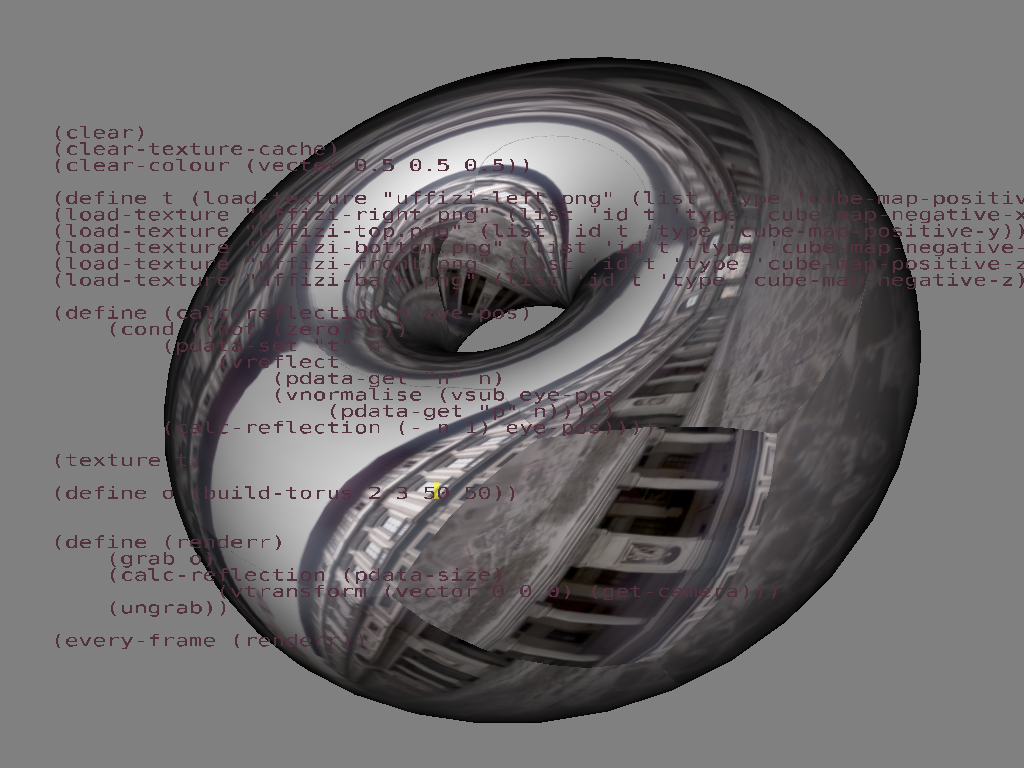
 (define t (load-texture "cube-left.png" (list 'type 'cube-map-positive-x)))
 (load-texture "cube-right.png" (list 'id t 'type 'cube-map-negative-x))
 (load-texture "cube-top.png" (list 'id t 'type 'cube-map-positive-y))
 (load-texture "cube-bottom.png" (list 'id t 'type 'cube-map-negative-y))
 (load-texture "cube-front.png" (list 'id t 'type 'cube-map-positive-z))
 (load-texture "cube-back.png" (list 'id t 'type 'cube-map-negative-z))
 (texture t)
Compressed textures
Compressed textures allow you to load more textures into less memory and can also improve texturing performance due to fewer memory accesses during texture filtering. (load-texture) reads DXT compressed texture files. To compress your textures there are a couple of options, for example nvcompress from
NVIDIA's GPU-accelerated Texture Tools.
(clear)
(texture (load-texture "test.dds"))
(build-cube)
Lighting
We have got away so far with ignoring the important topic of lighting. This is because there is a default light provided in fluxus, which is pure white and is attached to the camera, so it always allows you to see primitives clearly. However, this is a very boring setup, and if you configure your lighting yourself, you can use lights in very interesting and creative ways, so it's good to experiment with what is possible.
The standard approach in computer graphics comes from photography, and is referred to as 3 point lighting. The three lights you need are:
- Key – the key light is the main light for illuminating the subject. Put this on the same side of the subject as the camera, but off to one side.
- Fill – the fill light removes hard shadows from the fill light and provides some diffuse lighting. Put this on the same side as the camera, but to the opposite side to the key light.
- Rim or Back light, to separate the subject from the background. Put this behind the subject, to one side to illuminate the edges of the subject.
Here is an example fluxus script to set up such a light arrangement:
; light zero is the default camera light
; set to a low level
(light-diffuse 0 (vector 0 0 0))
(light-specular 0 (vector 0 0 0))

; make a big fat key light
(define key (make-light 'spot 'free))
(light-position key (vector 5 5 0))
(light-diffuse key (vector 1 0.95 0.8))
(light-specular key (vector 0.6 0.3 0.1))
(light-spot-angle key 22)
(light-spot-exponent key 100)
(light-direction key (vector -1 -1 0))

; make a fill light
(define fill (make-light 'spot 'free))
(light-position fill (vector -7 7 12))
(light-diffuse fill (vector 0.5 0.3 0.1))
(light-specular fill (vector 0.5 0.3 0.05))
(light-spot-angle fill 12)
(light-spot-exponent fill 100)
(light-direction fill (vector 0.6 -0.6 -1))

; make a rim light
(define rim (make-light 'spot 'free))
(light-position rim (vector 0.5 7 -12))
(light-diffuse rim (vector 0 0.3 0.5))
(light-specular rim (vector 0.4 0.6 1))
(light-spot-angle rim 12)
(light-spot-exponent rim 100)
(light-direction rim (vector 0 -0.6 1))
Shadows
The lack of shadows is a big problem with computer graphics. They are complex and time consuming to generate, but add so much to a feeling of depth and form.
However, they are quite easy to add to a fluxus scene:
(clear)
(light-diffuse 0 (vector 0 0 0)) ; turn the main light off
(define l (make-light 'point 'free)) ; make a new light
(light-position l (vector 10 50 50)) ; move it away
(light-diffuse l (vector 1 1 1))
(shadow-light l) ; register it as the shadow light

(with-state
    (translate (vector 0 2 0))
    (hint-cast-shadow) ; tell this primitive to cast shadows
    (build-torus 0.1 1 10 10))

(with-state ; make something for the shadow to fall onto.
    (rotate (vector 90 0 0))
    (scale 10)
    (build-plane))
Problems with shadows
There are some catches with the use of shadows in fluxus. Firstly they require some extra data to be generated for the primitives that cast shadows. This can be time consuming to calculate for complex meshes - although it will only be calculated the first time a primitive is rendered (usually the first frame).
A more problematic issue is a side effect of the shadowing method fluxus uses, which is fast and accurate, but won't work if the camera itself is inside a shadow volume. You'll see shadows disappearing or inverting. It can take some careful scene set up to avoid this happening.
A common alternatives to calculated shadows (or lighting in general) is to paint them into textures, this is a much better approach if the light and objects are to remain fixed.

Render Hints
We've already come across some render hints, but to explain them properly, they are miscellaneous options that can change the way a primitive is rendered. These options are called hints, as for some types of primitives they may not apply, or may do different things. They are useful for debugging, and sometimes just for fun.
(hint-none)
This is a very important render hint – it clears all other hints. By default only one is set – hint-solid. If you want to turn this off, and just render a cube in wire frame (for instance) you'd need to do this:
(hint-none)
(hint-wire)
(build-cube)
For a full list of the render hints, see the function reference section. You can do some pretty crazy things, for instance:
(clear)
(light-diffuse 0 (vector 0 0 0))
(define l (make-light 'point 'free))
(light-position l (vector 10 50 50))
(light-diffuse l (vector 1 1 1))
(shadow-light l)

(with-state
    (hint-none)
    (hint-wire)
    (hint-normal)
    (translate (vector 0 2 0))
    (hint-cast-shadow)
    (build-torus 0.1 1 10 10))

(with-state
    (rotate (vector 90 0 0))
    (scale 10)
    (build-plane))
Draws the torus from the shadowing example but is rendered in wireframe, displaying it's normals as well as casting shadows. It's become something of a fashion to find ways of using normals rendering creatively in fluxus!
About Primitives
Primitives are objects that you can render. There isn’t really much else in a fluxus scene, except lights, a camera and lots of primitives.
Primitive state
The normal way to create a primitive is to set up some state which the primitive will use, then call it’s build function and keep it’s returned ID (using with-primitive) to modify it’s state later on.
(define myobj (with-state
                (colour (vector 0 1 0))
                (build-cube))) ; makes a green cube

(with-primitive myobj
        (colour (vector 1 0 0))) ; changes its colour to red
So primitives contain a state which describes things like colour, texture and transform information. This state operates on the primitive as a whole – one colour for the whole thing, one texture, shader pair and one transform. To get a little deeper and do more we need to introduce primitive data.
Primitive Data Arrays [aka. Pdata]
 A pdata array is a fixed size array of information contained within a primitive. Each pdata array has a name, so you can refer to it, and a primitive may contain lots of different pdata arrays (which are all the same size). Pdata arrays are typed – and can contain floats, vectors, colours or matrices. You can make your own pdata arrays, with names that you choose, or copy them in one command.
Some pdata is created when you call the build function. This automatically generated pdata is given single character names. Sometimes this automatically created pdata results in a primitive you can use straight away (in commands such as build-cube) but some primitives are only useful if pdata is setup and controlled by you.
In polygons, there is one pdata element per vertex – and a separate array for vertex positions, normals, colours and texture coordinates.
So, for example <code>(build-sphere)</code> creates a polygonal object with a spherical distribution of vertex point data, surface normals at every vertex and texture coordinates, so you can wrap a texture around the primitive. This data (primitive data, or pdata for short) can be read and written to inside a with-primitive corresponding to the current object.
(pdata-set! name vertnumber vector)
Sets the data on the current object to the input vector
(pdata-ref name vertnumber)
Returns the vector from the pdata on the current object
(pdata-size)
Returns the size of the pdata on the current object (the number of vertices).
The name describes the data we want to access, for instance “p” contains the vertex positions:
(pdata-set! “p” 0 (vector 0 0 0))
Sets the first point in the primitive to the origin (not all that useful)
(pdata-set! “p” 0 (vadd (pdata-ref “p” 0) (vector 1 0 0)))
The same, but sets it to the original position + 1 in the x offsetting the position is more useful as it constitutes a deformation of the original point. (See Deforming, for more info on deformations)
Mapping, Folding
The pdata-set! and pdata-ref procedures are useful, but there is a more powerful way of deforming primitives. Map and fold relate to the scheme functions for list processing, it’s probably a good idea to play with them to get a good understanding of what these are doing.
(pdata-map! Procedure read/write-pdata-name read-pdata-name ...)
Maps over pdata arrays – think of it as a for-every pdata element, and writes the result of procedure into the first pdata name array.
An example, using pdata-map to invert normals on a primitive:
(define p (build-sphere 10 10))

(with-primitive p
(pdata-map!
        (lambda (n)
                (vmul n -1))
        "n"))
This is more concise and less error prone than using the previous functions and setting up the loop yourself.
(pdata-index-map! Procedure read/write-pdata-name read-pdata-name ...)
Same as pdata-map! but also supplies the current pdata index number to the procedure as the first argument.
(pdata-fold procedure start-value read-pdata-name read-pdata-name ...)
This example calculates the centre of the primitive, by averaging all it’s vertex positions together:
(define my-torus (build-torus 1 2 10 10))
(define torus-centre
        (with-primitive my-torus
                (vdiv (pdata-fold vadd (vector 0 0 0) “p”) (pdata-size)))))
(pdata-index-fold procedure start-value read-pdata-name read-pdata-name ...)
Same as pdata-fold but also supplies the current pdata index number to the procedure as the first argument.
Instancing
Sometimes retained mode primitives can be unwieldy to deal with. For instance, if you are rendering thousands of identical objects, or doing things with recursive graphics, where you are calling the same primitive in lots of different states – keeping track of all the Ids would be annoying to say the least.
This is where instancing is helpful, all you call is:
(draw-instance myobj)
Will redraw any given object in the current state (immediate mode). An example:
(define myobj (build-nurbs-sphere 8 10)) ; make a sphere

(define (render-spheres n)
        (cond ((not (zero? n))
                (with-state
                (translate (vector n 0 0)) ; move in x
                (draw-instance myobj))     ; stamp down a copy
                (render-spheres (- n 1)))))    ; recurse!

(every-frame (render-spheres 10)) ; draw 10 copies
Built In Immediate Mode Primitives
To make life even easier than having to instance primitives, there are some built in primitives that can be rendered at any time, without being built:
(draw-cube)
(draw-sphere)
(draw-plane)
(draw-cylinder)
For example:
(define (render-spheres n)
        (cond ((not (zero? n))
                (with-state
                        (translate (vector n 0 0)) ; move in x
                        (draw-sphere))             ; render a new sphere
                (render-spheres (- n 1)))))    ; recurse!

(every-frame (render-spheres 10)) ; draw 10 copies
These built in primitives are very restricted in that you can’t edit them or change their resolution settings etc, but they are handy to use for quick scripts with simple shapes.
Somebody Should Set The Title For This Chapter!
Primitives are the most interesting things in fluxus, as they are the things which actually get rendered and make up the scene.
Polygon Primitive
 Polygon primitives are the most versatile primitives, as fluxus is really designed around them. The other primitives are added in order to achieve special effects and have specific roles. The other primitive types often have commands to convert them into polygon primitives, for further processing.
There are many commands which create polygon primitives:
(build-cube)
(build-sphere 10 10)
(build-torus 1 2 10 10)
(build-plane)
(build-seg-plane 10 10)
(build-cylinder 10 10)
(build-polygons 100 'triangles)
The last one is useful if you are building your own shapes from scratch, the others are useful for giving you some preset shapes. All build-* functions return an id number which you can store and use to modify the primitive later on.
Pdata Types
The pdata arrays available for polygons are as follows:
Vertex normal n 3 vector Vertex texture coords t 3 vector for u and v, the 3rd number is ignored Vertex colours c 4 vector rgba
| Use |
Name |
Data Type |
| Vertex position |
p |
3 vector |
| Vertex normal |
n |
3 vector |
| Vertex texture coords |
t |
3 vector for u and v, the 3rd number is ignored |
| Vertex colours |
c |
4 vector rgba |
Polygon topology and pdata
With polygonal objects, we need to connect the vertices defined by the pdata into faces that describe a surface. The topology of the polygon primitive sets how this happens:
Quad-list topology
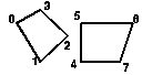
Triangle-list topology
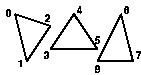
Triangle-strip topology
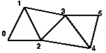
Triangle-fan topology
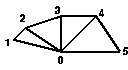
Polygon topology

This lookup is the same for all the pdata on a particular polygon primitive - vertex positions, normals, colours and texture coordinates.
Although using these topologies means the primitive is optimised to be very quick to render, it costs some memory as points are duplicated - this can also cause a big speed impact if you are doing lots of per-vertex calculation. The most optimal poly topology are triangle strips as they maximise the sharing of vertices, but also see indexed polygons for a potentially even faster method.
You can find out the topology of a polygon primitive like this:
(define p (build-cube))

(with-primitive p
    (display (poly-type))(newline)) ; prints out quad-list
Indexed polygons
The other way of improving efficiency is converting polygons to indexed mode. Indexing means that vertices in different faces can share the same vertex data. You can set the index of a polygon manually with:
(with-primitive myobj
        (poly-set-index list-of-indices))
Or automatically – (which is recommended) with:
(with-primitive myobj
        (poly-convert-to-indexed))
This procedure compresses the polygonal object by finding duplicated or very close vertices and “gluing” them together to form one vertex and multiple index references. Indexing has a number of advantages, one that large models will take less memory - but the big deal is that deformation or other per-vertex calculations will be much quicker.
Problems with automatic indexing
As all vertex information becomes shared for coincident vertices, automatically indexed polygons can’t have different normals, colours or texture coordinates for vertices at the same position. This means that they will have to be smooth and continuous with respect to lighting and texturing. This should be fixed in time, with a more complicated conversion algorithm.
NURBS Primitives 
NURBS are parametric curved patch surfaces. They are handled in a similar way to polygon primitives, except that instead of vertices, pdata elements represent control vertices of the patch. Changing a control vertex causes the mesh to smoothly blend the change across it’s surface.
(build-nurbs-sphere 10 10)
(build-nurbs-plane 10 10)
Pdata Types
| Use |
Name |
Data Type |
| Control vertex position |
p |
3 vector |
| Control vertex texture coords |
t |
3 vector for u and v, the 3rd number is ignored |
| Control vertex colours |
c |
4 vector rgba |
Particle primitive 
Particle primitives use the pdata elements to represent a point, or a camera facing sprite which can be textured – depending on the render hints. This primitive is useful for lots of different effects including, water, smoke, clouds and explosions.
(build-particles num-particles)
| Use |
Name |
Data Type |
| Particle position |
p |
3 vector |
| Particle colour |
c
|
3 vector |
| Particle size |
s
|
3 vector for width and height, the 3rd number is ignored |
Geometry hints
Particle primitives default to camera facing sprites, but can be made to render as points in screen space, which look quite different. To switch to points:
(with-primitive myparticles
    (hint-none)    ; turns off solid, which is default sprite mode
    (hint-points)) ; turn on points rendering
If you also enable (hint-anti-alias) you may get circular points, depending on your GPU – these can be scaled in pixel space using (point-width).
Ribbon primitives
Ribbon primitives are similar to particles in that they are either hardware rendered lines or camera facing textured quads. This primitive draws a single line connecting each pdata vertex element together. The texture is stretched along the ribbon from the start to the end, and width wise across the line. The width can be set per vertex to change the shape of the line.
(build-ribbon num-points)
Pdata Types
Use
|
Name
|
Data Type
|
Ribbon vertex position
|
p
|
3 vector
|
Ribbon vertex colour
|
c
|
3 vector
|
Ribbon vertex width
|
w
|
number
|
Geometry hints
Ribbon primitives default to render camera facing quads. You can also switch them to draw wire frame lines in screen space:
(with-primitive myline
    (hint-none) ; turns off solid, which is default mode
    (hint-wire)) ; turn on lines rendering
Text primitive
Text primitives allow you to create text based on texture fonts. The font assumed to be non proportional – there is an example font shipped with fluxus.
(texture (load-texture “font.png”))
(build-text text-string)
The primitive makes a set of quads, one for each character, with texture coordinates set to show the correct character from the texture. This provides a fast and cheap way of displaying text, and is useful for debugging, or if the text is quite small. You can probably also find quite creative ways of using this just as a way of chopping up a texture into little squares.
Type Primitive
The type primitive provides a much higher quality typeface rendering than the text primitive. It creates polygonal geometry from a ttf font and some text. Optionally you can also extrude the text which results in 3D shapes.
(build-type ttf-font-filename text)
(build-extruded-type ttf-font-filename text
extrude depth)
You can also convert the type primitive into a polygon primitive for further deformation or applying textures, with:
(type->poly type-prim-id)
Locator primitive
The locator is a null primitive, as it doesn’t render anything. Locators are useful for various tasks, you can use them as a invisible scene node to group primitive under. They are also used to build skeletons for skinning. To view them, you can turn on hint-origin, which draws an axis representing their transform.
(hint-origin)
(build-locator)
Pixel primitive
A pixel primitive is used for making procedural textures, which can then be applied to other primitives. For this reason, pixel primitives probably wont be rendered much directly, but you can render them to preview the texture on a flat plane.
(pixel-primitive width height)
| Use |
Name |
Data Type
|
Pixel colour
|
c
|
3 vector
|
Pixel alpha
|
a
|
number
|
Extra pixel primitive commands
A pixel primitive’s pdata corresponds to pixel values in a texture, you write to them to make procedural texture data. The pixel primitive comes with some extra commands:
(pixels-upload pixelprimitiveid-number)
Uploads the texture data, you need to call this when you’ve finished writing to the pixelprim, and while it’s grabbed.
(pixels->texture pixelprimitiveid-number)
Returns a texture you can use exactly like a normal loaded one.
See the examples for some procedural texturing. It’s important to note that creating textures involves a large amount of processing time, so you don’t want to plan on doing something per-pixel/per-frame for large textures. The pdata-func extensions could be used to help here in the future.
This is a simple example of creating a noise texture on a pixel primitive:
(with-primitive (build-pixels 100 100)
    (pdata-map!
        (lambda (colour)
            (rndvec))
        "c")
    (pixels-upload))
Blobby Primitives
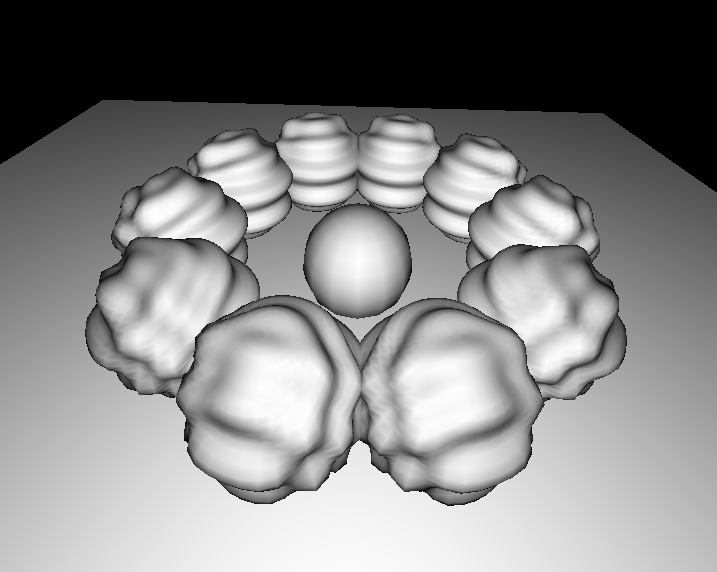
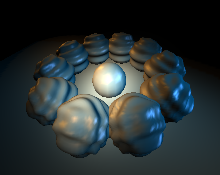
Blobby primitives are a higher level implicit surface representation in fluxus which is defined using influences in space. These influences are summed together, and a particular value is “meshed” (using the marching cubes algorithm) to form a smooth surface. The influences can be animated, and the smooth surface moves and deforms to adapt, giving the primitive it’s blobby name. (build-blobby) returns a new blobby primitive id. Numinfluences is the number of “blobs”. Subdivisions allows you to control the resolution of the surface in each dimension, while boundingvec sets the bounding area of the primitive in local object space. The mesh will not be calculated outside of this area. Influence positions and colours need to be set using pdata-set.
(build-blobby numinfluences subdivisionsvec boundingvec)
Pdata Types
| Use |
Name |
Data Type
|
| Position |
p |
3 vecor
|
| Strengh |
s |
number |
| Colour |
c |
3 vector
|
Converting to polygons
Blobbies can be slow to calculate, if you only need static meshes without animation, you can convert them into polygon primitives with:
(blobby->poly blobby-id-num)
Deforming
Deformation in this chapter signifies various operations. It can involve changing the shape of a primitive in a way not possible via a transform (i.e. bending, warping etc) or modifying texture coordinates or colours to achieve a per-vertex effect. Deformation in this way is also the only way to get particle primitives to do anything interesting.
Deforming is all about pdata, so, to deform an entire object, you do something like the following:
(clear)
(hint-none)
(hint-wire)
(line-width 4)

(define myobj (build-sphere 10 10))

(with-primitive myobj
    (pdata-map!
        (lambda (p)
            ; add a small random vector to the original point
            (vadd (vmul (rndvec) 0.1) p))
        "p"))
When deforming geometry, moving the positions of the vertices is not usually enough, the normals will need to be updated for the lighting to work correctly.
(recalc-normals smooth)
Will regenerate the normals for polygon and nurbs primitives based on the vertex positions. Not particularly fast (it is better to deform the normals in your script if you can). If smooth is 1, the face normals are averaged with the coincident face normals to give a smooth appearance.
When working on polygon primitives fluxus will cache certain results, so it will be a lot slower on the first calculation than subsequent calls on the same primitive.
User Pdata 
As well as the standard information that exists in primitives, fluxus also allows you to add your own per vertex data to any primitive. User pdata can be written or read in the same way as the built in pdata types.
(pdata-add name type)
Where name is a string with the name you wish to call it, and type is a one character string consisting of:
f : float data
v : vector data
c : colour data
m : matrix data
(pdata-copy source destination)
This will copy a array of pdata, or overwrite an existing one with if it already exists. Adding your own storage for data on primitives means you can use it as a fast way of reading and writing data, even if the data doesn’t directly affect the primitive.
An example of a particle explosion:
; setup the scene
(clear)
(show-fps 1)
(point-width 4)
(hint-anti-alias)

; build our particle primitive
(define particles (build-particles 1000))

; set up the particles
(with-primitive particles
    (pdata-add "vel" "v") ; add the velocity user pdata of type vector
    (pdata-map! ; init the velocities
        (lambda (vel)
            (vmul (vsub (vector (flxrnd) (flxrnd) (flxrnd))
                        (vector 0.5 0.5 0.5)) 0.1))
        "vel")
    (pdata-map! ; init the colours
        (lambda (c)
            (vector (flxrnd) (flxrnd) 1))
        "c"))

(blur 0.1)

; a procedure to animate the particles
(define (animate)
    (with-primitive particles
        (pdata-map!
            (lambda (vel)
                (vadd vel (vector 0 -0.001 0)))
            "vel")
        (pdata-map! vadd "p" "vel")))

(every-frame (animate))
Pdata Operations
Pdata Operations are a optimisation which takes advantage of the nature of these storage arrays to allow you to process them with a single call to the scheme interpreter. This makes deforming primitive much faster as looping in the scheme interpreter is slow, and it also simplifies your scheme code.
(pdata-op operation pdata operand)
Where operation is a string identifier for the intended operation (listed below) and pdata is the name of the target pdata to operate on, and operand is either a single data (a scheme number or vector (length 3,4 or 16)) or a name of another pdata array.
If the (update) and (render) functions in the script above are changed to the following:
(define (update)
    ; add this vector to all the velocities
    (pdata-op "+" "vel" (vector 0 -0.002 0))
    ; add all the velocities to all the positions
    (pdata-op "+" "p" "vel"))

(define (render)
    (with-primitive ob
        (update)))
On my machine, this script runs over 6 times faster than the first version.
(pdata-op) can also return information to your script from certain functions called on entire pdata arrays.
Pdata operations
“+” : addition
“*” : multiplication
“sin” : writes the sine of one float pdata array into another “cos” : writes the cosine of one float pdata array into another “closest” : treats the vector pdata as positions, and if given a single vector, returns the closest position to it – or if given a float, uses it as a index into the pdata array, and returns the nearest position.
For most pdata operations, the vast majority of the combinations of input types (scheme number, the vectors or pdata types) will not be supported, you will receive a rather cryptic runtime warning message if this is the case.
Pdata functions
Pdata ops are useful, but I needed to expand the idea into something more complicated to support more interesting deformations like skinning. This area is messy, and somewhat experimental – so bear with me, it should solidify in future.
Pdata functions (pfuncs) range from general purpose to complex and specialised operations which you can run on primitives. All pfuncs share the same interface for controlling and setting them up. The idea is that you make a set of them at startup, then run them on one or many primitives later on per-frame.
(make-pfunc pfunc-name-symbol))
Makes a new pfunc. Takes the symbol of the names below, e.g. (make-pfunc ‘arithmetic)
(pfunc-set! pfuncid-number argument-list)
Sets arguments on a primitive function. The argument list consists of symbols and corresponding values.
(pfunc-run id-number)
Runs a primitive function on the current primitive. Look at the skinning example to see how this works.
Pfunc types
All pfunc types and arguments are as follows:
arithmetic
For applying general arithmetic to any pdata array
operator string : one of: add sub mul div
src string : pdata array name
other string : pdata array name (optional)
constant float : constant value (optional)
dst string : pdata array name
genskinweights
Generates skinweights – adds float pdata called “s1” -> “sn” where n is the number of nodes in the skeleton – 1
skeleton-root primid-number : the root of the bindpose skeleton for skinning sharpness float : a control of how sharp the creasing will be when skinned
skinweights->vertcols
A utility for visualising skinweights for debugging.
No arguments
skinning
Skins a primitive – deforms it to follow a skeleton’s movements. Primitives we want to run this on have to contain extra pdata – copies of the starting vert positions called “pref” and the same for normals, if normals are being skinned, called “nref”.
Skeleton-root primid-number : the root primitive of the animating skeleton bindpose-root primid-number : the root primitive of the bindpose skeleton skin-normals number : whether to skin the normals as well as the positions
Using Pdata to build your own primitives
The function (build_polygons) allows you to build empty primitives which you can use to either build more types of procedural shapes than fluxus supports naively, or for loading model data from disk. Once these primitives have been constructed they can be treated in exactly the same way as any other primitive, ie pdata can be added or modified, and you can use (recalc-normals) etc.
Cameras
Without a camera you wouldn't be able to see anything! They are obviously very important in 3D computer graphics, and can be used very effectively, just like a real camera to tell a story.
Moving the camera
You can already control the camera with the the mouse, but sometimes you'll want to control the camera procedurally from a script. Animating the camera this way is also easy, you just lock it to a primitive and move that:
(clear)
(define obj (build-cube)) ; make a cube for the camera to lock to

(with-state ; make a background cube so we can tell what's happening
    (hint-wire)
    (hint-unlit)
    (texture (load-texture "test.png"))
    (colour (vector 0.5 0.5 0.5))
    (scale (vector -20 -10 -10))
    (build-cube))

(lock-camera obj) ; lock the camera to our first cube
(camera-lag 0.1) ; set the lag amount, this will smooth out the cube jittery movement

(define (animate)
    (with-primitive obj
         (identity)
         (translate (vector (fmod (time) 5) 0 0)))) ; make a jittery movement

(every-frame (animate))
Stopping the mouse moving the camera
The mouse camera control still works when the camera is locked to a primitive, it just moves it relative to the locked primitive. You can stop this happening by setting the camera transform yourself:
set-camera-transform (mtranslate (vector 0 0 -10)))
This command takes a transform matrix (a vector of 16 numbers) which can be generated by the maths commands (mtranslate), (mrotate) and (mscale) and multiplied together with (mmul).
You just need to call (set-camera-transform) once, it gives your script complete control over the camera, and frees the mouse up for doing other things.. To switch mouse movement back on, use:
(reset-camera)
More camera properties
 By default the camera is set to perspective projection. To use orthographic projection just use:
(ortho)
Moving the camera back and forward has no effect with orthographic projection, so to zoom the display, use:
(set-ortho-zoom 10)
And use:
(persp)
To flip the camera back to perspective mode.
The camera angle can be changed with the rather confusingly named command:
(clip 1 10000)
Which sets the near and far clipping plane distance. The far clipping plane (the second number) sets where geometry will start getting dropped out. The first number is interesting to us here as it sets the distance from the camera centre point to the near clipping plane. The smaller this number, the wider the camera angle.
Fogging
Not strictly a camera setting, but fog fades out objects as they move away from the camera - giving the impression of aerial perspective.
(fog (vector 0 0 1) 0.01 1 1000)
The first number is the colour of the fog, followed by the strength (keep it low) then the start and end of the fogging (which don't appear to work on my graphics card, at least).
Fog used to be used as a way of hiding the back clipping plane, or making it slightly less jarring, so things fade away rather than disappear - however it also adds a lot of realism to outdoor scenes, and I'm a big fan of finding more creative uses for it.
Using multiple cameras
Todo: hiding things in different camera views
Noise and Randomness
Noise and randomness is used in computer animation in order to add “dirt” to your work. This is very important, as the computer is clean and boring by default.
Randomness
Scheme has it's own built in set of random operations, but Fluxus comes with a set of it's own to make life a bit easier for you.
Random number operations
These basic random commands return numbers:
(rndf) ; returns a number between 0 and 1
(crndf) ; (centred) returns a number between -1 and 1
(grndf) ; returns a Gaussian random number centred on 0 with a variance of 1
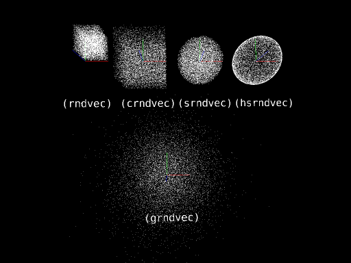
Random vector operations
More often than not, when writing fluxus scripts you are interested in getting random vectors, in order to perturb or generate random positions in space, directions to move in, or colours.
(rndvec) ; returns a vector where the elements are between 0 and 1
(crndvec) ; returns a vector where the elements are between -1 and 1
(srndvec) ; returns a vector represented by a point inside a sphere of radius 1
(hsrndvec) ; a vector represented by a point on the surface of a sphere radius 1, hollow sphere
(grndvec) ; a Gaussian position centred on 0,0,0 with variance of 1
These are much better described by a picture:
Noise
todo
Scene Inspection
So far we have mostly looked at describing objects and deformations to fluxus so it can build scenes for you. Another powerful technique is to get fluxus to inspect your scene and give you information on what is there.
Scene graph inspection
 The simplest, and perhaps most powerful commands for inspection are these commands:
(get-children)
(get-parent)
(get-children) returns a list of the children of the current primitive, it can also give you the list of children of the scene root node if you call it outside of (with-primitive). (get-parent) returns the parent of the current primitive. These commands can be used to navigate the scenegraph and find primitives without you needing to record their Ids manually. For instance, a primitive can change the colour of it's parent like this:
(with-primitive myprim
        (with-primitive (get-parent)
                (colour (vector 1 0 0))))
You can also visit every primitive in the scene with the following script:
; navigate the scene graph and print it out
(define (print-heir children)
    (for-each
        (lambda (child)
            (with-primitive child
                (printf "id: ~a parent: ~a children: ~a~n" child (get-parent) (get-children))
                (print-heir (get-children))))
        children))
Collision detection
A very common thing you want to do is find out if two objects collide with each other (particularly when writing games). You can find out if the current primitive roughly intersects another one with this command:
(bb/bb-intersect? other-primitive box-expand)
This uses the automatically generated bounding box for the primitives, and so is quite fast and good enough for most collision detection. The box expand value is a number with which to add to the bounding box to expand or shrink the volume it uses for collision detection.
Note: The bounding box used is not the same one as you see with (hint-box), which is affected by the primitive's transform. bb-intersect generates new bounding boxes which are all axis aligned for speed of comparison.
Ray Casting
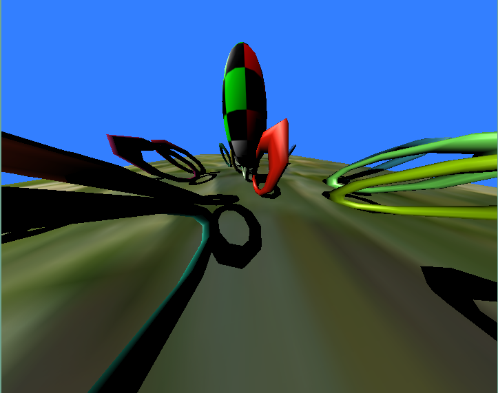
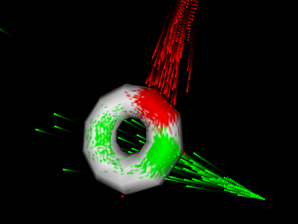
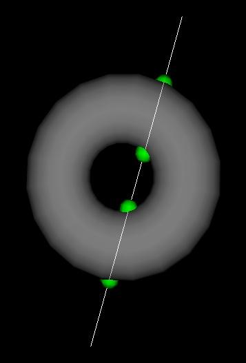 Another extremely useful technique is to create rays, or lines in the scene and get information about where on primitives they intersect with. This can be used for detailed collision detection or in more complex techniques like raytracing.
(geo/line-intersect line-start-position line-end-position)
This command returns a list of pdata values at the points where the line intersects with the current primitive. The clever thing is that it values for the precise intersection point – not just the closest vertex.
The list it returns is designed to be accessed using Scheme (assoc) command. An intersection list looks like this:
(collision-point-list collision-point-list ...)
Where a collision point list looks like:
(("p" . position-vector) ("t" . texture-vector) ("n" . normal-vector) ("c" . colour-vector))
The green sphere in the illustration are positioned on the "p" pdata positions returned by the following snippet of code:
(clear)

(define s (build-torus 1 2 10 10))

; line endpoint positions
(define a (vector 3 2.5 1))
(define b (vector -2 -3 -.1))

; draw the line
(with-primitive (build-ribbon 2)
    (hint-wire)
    (hint-unlit)
    (pdata-set! "p" 0 a)
    (pdata-set! "p" 1 b))

; process intersection point list
(with-primitive s
    (for-each
      (lambda (intersection)
        (with-state ; draw a sphere at the intersection point
          (translate (cdr (assoc "p" intersection)))
          (colour (vector 0 1 0))
          (scale (vector 0.3 0.3 0.3))
          (build-sphere 5 5)))
      (geo/line-intersect a b)))
Primitive evaluation
poly-for-each-face
poly-for-each-triangle
poly-for-each-tri-sample
Primitive Loading and Saving
It's useful to be able to load and save primitives, this is for several reasons. You may wish to use other programs to make meshes and import them into fluxus, or to export primitives you've made in fluxus to render them in other programs. It's also useful to save the primitive as a file if the process to create it in fluxus is very slow. There are only two commands you need to know to do this:
; load a primitive in:
(define newprim (load-primitive filename))
; save it out again:
(with-primitive newprim
        (save-primitive filename))
At present these commands work on poly and pixel primitives, and load/save obj and png files respectively.
COLLADA format support
 Collada is a standard file format for complex 3D scenes. Collada files can be loaded, currently supported geometry is triangular data, vertex positions, normals and texture coordinates. The plan is to use collada for complex scenes containing different geometry types, including animation and physics data.
(collada-import filename)
(collada-import) loads a collada scene file and returns a scene description list. Files need to contain triangulated model data - this is usually an option on the export. Note: this is slow for heavy models.
Shaders
Hardware shaders allow you to have much finer control over the graphics pipeline used to render your objects. Fluxus has commands to set and control GLSL shaders from your scheme scripts, and even edit your shaders in the fluxus editor. GLSL is the OpenGL standard for shaders across various graphics card types, if your card and driver support OpenGL2, this should work for you.
(shader vertshader fragshader)
Loads, compiles and binds the vertex and fragment shaders on to current state or grabbed primitive.
(shader-set! paramlist)
Sets uniform parameters for the shader in a token, value list, e.g.:
(list “specular” 0.5 “mycolour” (vector 1 0 0))
This is very simple to set up – in your GLSL shader you just need to declare a uniform value eg:
uniform float deformamount;
This is then set by calling from scheme:
(shader-set! (list “deformamount” 1.4))
The deformamount is set once per object/shader – hence it’s a uniform value across the whole object. Shaders also get given all pdata as attribute (per vertex) parameters, so you can share all this information between shaders and scripts in a similar way:
In GLSL:
attribute vec3 testcol;
To pass this from scheme, first create some new pdata with a matching name:
(pdata-add “testcol” “v”)
Then you can set it in the same way as any other pdata, controlling shader parameters on a per-vertex basis.
Samplers
Samplers are the hardware shading word for textures, the word sampler is used to be a little more general in that they are used as a way of passing lots of information (which may not be visual in nature) around between shaders. Passing textures into GLSL shaders from fluxus is again fairly simple:
In your GLSL shader:
uniform sampler2D mytexture;
In scheme:
(texture (load-texture “mytexturefile.png”))
(shader-set! (list “mytexture” 0))
This just tells GLSL to use the first texture unit (0) as the sampler for mytexture. This is the texture unit that the standard (texture) command loads textures to.
To pass more than one texture, you need multitexturing turned on:
In GLSL:
uniform sampler2D mytexture;
uniform sampler2D mysecondtexture;
In scheme:
; load to texture unit 0
(multitexture 0 (load-texture “mytexturefile.png”))
; load to texture unit 1
(multitexture 1 (load-texture “mytexturefile2.png”))
(shader-set! (list “mytexture” 0 “mysecondtexture” 1))
Turtle Builder
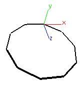
The turtle polybuilder is an experimental way of building polygonal objects using a logo style turtle in 3D space. As you drive the turtle around you can place vertices and build shapes procedurally. The turtle can also be used to deform existing polygonal primitives, by attaching it to objects you have already created.
This script simply builds a single polygon circle, by playing the age old turtle trick of looping a function that moves a bit, turns a bit...
(clear)

(define (build n)
    (turtle-reset)
    (turtle-prim 4)
    (build-loop n n)
    (turtle-build))

(define (build-loop n t)
    (turtle-turn (vector 0 (/ 360 t) 0))
    (turtle-move 1)
    (turtle-vert)
    (if (< n 1)
        0
        (build-loop (- n 1) t)))

(backfacecull 0)
(hint-unlit)
(hint-wire)
(wire-colour (vector 0 0 0))
(line-width 4)
(build 10)
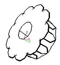 For a more complex example, just modify the
 (build-loop) function as so:
(define (build-loop n t)
    (turtle-turn (vector 0 (/ 360 t) 0))
    (turtle-move 1)
    (turtle-vert)
    (if (< n 1)
         0
         (begin
             ; add another call to the recursion
             (build-loop (- n 1) t)
             (turtle-turn (vector 0 0 45))   ; twist a bit
             (build-loop (- n 1) t))))
Notes on Writing Large Programs in Fluxus
When writing large programs in fluxus, I've found that there are some aspects of the language (the PLT scheme dialect to be more precise) which are essential in managing code and keeping things tidy. See the PLT documentation on structs and classes for more detail, but I'll give some fluxus related examples to work with.
For example, at first we can get along quite nicely with using lists alone to store data. Let's use as an example a program with a robot we wish to control:
(define myrobot (list (vector 0 0 0) (vector 1 0 0) (build-cube)))
We use a list to store the robot's position, velocity and a primitive associated with it. We could then use:
(list-ref myrobot 0) ; returns the position of the robot
(list-ref myrobot 1) ; returns the velocity of the robot
(list-ref myrobot 2) ; returns the root primitive of the robot
To get at the values of the robot and use them later. Seems pretty handy, but this has problems when we scale up the problem, say we want to make a world to keep our robots in:
; build a world with three robots
(define world (list (list (vector 0 0 0) (vector 1 0 0) (build-cube))
        (list (vector 1 0 0) (vector 1 0 0) (build-cube))
        (list (vector 2 0 0) (vector 1 0 0) (build-cube)))
And then say we want to access the 2nd robot's root primitive:
(list-ref (list-ref world 1) 2)
It all starts to get a little confusing, as we are indexing by number.
Structs
Structs are simple containers that allow you to name data. This is a much saner way of dealing with containers of data than using lists alone.
Let's start again with the robots example:
(define-struct robot (pos vel root))
Where “pos” is the current position of the robot, “vel” it's velocity and “root” is the primitive for the robot. The (define-struct) automatically generates the following functions we can immediately use:
(define myrobot (make-robot (vector 0 0 0) (vector 0 0 0) (build-cube)) ; returns a new robot
(robot-pos myrobot) ; returns the position of the robot
(robot-vel myrobot) ; returns the velocity of the robot
(robot-root myrobot) ; returns the root primitive for the robot
This makes for very readable code, as all the data has meaning, no numbers to decipher. It also means we can insert new data and not have to rewrite a lot of code, which is very important.
The world can now become:
(define-struct world (robots))
And be used like this:
; build a world with three robots
(define myworld (make-world (list (make-robot (vector 0 0 0) (vector 1 0 0) (build-cube))
        (make-robot (vector 1 0 0) (vector 1 0 0) (build-cube))
        (make-robot (vector 2 0 0) (vector 1 0 0) (build-cube)))))

; get the 2nd robot's root primitive:
(robot-root (list-ref (world-robots myworld) 1))
Mutable state
So far we have only used get's not set's. This is partly because setting state is seen as slightly distasteful in Scheme, so you have to use the following syntax to enable it in a struct:
(define-struct robot ((pos #:mutable) (vel #:mutable) root))
This (define-struct) also generates the following functions:
(set-robot-pos! robot (vector 1 0 0))
(set-robot-vel! robot (vector 0 0.1 0))
So you can change the values in the program. For a full example, see the file dancing-robots.scm in the examples directory.
Classes
Making Movies
Fluxus is designed for real-time use, this means interactive performance or games mainly, but you can also use the frame dump commands to save out frames which can be converted to movies. This process can be fairly complex, if you want to sync visuals to audio, osc or keyboard input.
Used alone, frame dumping will simply save out frames as fast as your machine can render and save them to disk. This is useful in some cases, but not if we want to create a movie at a fixed frame rate, but with the same timing as they are generated at – ie synced with an audio track at 25fps.
Syncing to audio
The (process) command does several things, it switches the audio from the jack input source to a file, but it also makes sure that every buffer of audio is used to produce exactly one frame. Usually in real-time operation, audio buffers will be skipped or duplicated, depending on the variable frame rate and fixed audio rate.
So, what this actually means is that if we want to produce video at 25fps, with audio at 44100 samplerate, 44100/25 = 1764 audio samples per frame. Set your (start-audio) buffer setting to this size. Then all you need to do is make sure the calls to (process) and (start-framedump) happen on the same frame, so that the first frame is at the start of the audio. As this process is not real-time, you can set your resolution as large as you want, or make the script as complex as you like.
Syncing with keyboard input for livecoding recordings
You can use the keypress recorder to save livecoding performances and rerender them later.
To use the key press recorder, start fluxus with -r or -p (see in-fluxus docs for more info). It records the timing of each keypress to a file, it can then replay them at different frame rates correctly.
The keypress recorder works with the process command in the same way as the audio does (you always need an audio track, even if it’s silence). So the recorder will advance the number of seconds per frame as it renders, rather than using the real-time clock – so again, you can make the rendering as slow as you like, it will appear correct when you view the movie.
Recording OSC messages is also possible (for storing things like gamepad activity). Let me know if you want to do this.
Syncing Problems Troubleshooting
Getting the syncing right when combining audio input can be a bit tricky. Some common problems I’ve seen with the resulting movies fall into two categories.
Syncing lags, and gets worse with time
The call to (start-audio) has the wrong buffer size. As I set this in my .fluxus.scm I often forget this. Set it correctly and re-render. Some lagging may happen unavoidably with really long (over 20 minutes or so) animations.
Syncing is offset in a constant manner
This happens when the start of the audio does not quite match the first frame. You can try adding or removing some silence at the beginning of the audio track to sort this out. I often just encode the first couple of seconds until I get it right.
Fluxus in DrScheme
DrScheme is a “integrated development environment” for Scheme, and it comes as part of PLT scheme, so you will have it installed if you are using fluxus.
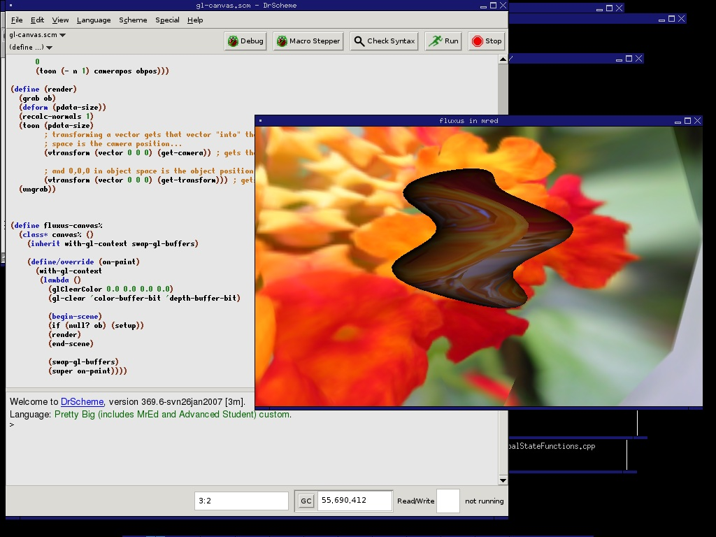 You can use it instead of the built in fluxus scratchpad editor for writing scheme scripts. Reasons to want to do this include:
- The ability to profile and debug scheme code
- Better editing environment than the fluxus scratchpad editor will ever provide
- Makes fluxus useful in more ways (with the addition of widgets, multiple views etc)
I use it a lot for writing larger scheme scripts. All you need to do is add the following line to the top of your fluxus script:
(require fluxus-[version]/drflux)
Where [version] is the current version number without the dot, eg “017”.
Load the script into DrScheme and press F5 to run it – a new window should pop up, displaying your graphics as normal. Rerunning the script in DrScheme should update the graphics window automatically.
DrScheme in OS X
If you put the fluxus binary application to /Applications, you need to include the resources folder of the fluxus.app to the collects path, so DrScheme finds the fluxus modules. because they depend on the dynamic libraries and frameworks included in the application, you also need to set the dynamic library path. something like this from terminal:
export PLTCOLLECTS=/Applications/PLT\ Scheme\ v4.2.5/collects/:/Applications/Fluxus.app/Contents/Resources/collects/
export DYLD_LIBRARY_PATH=/Applications/Fluxus.app/Contents/Frameworks/
then load DrScheme:
open /Applications/PLT\ Scheme\ v4.2.5/DrScheme.app/
a simple test script should work now:
#lang scheme
(require fluxus-[version]/drflux)
(clear)
(build-cube)
Where [version] is the current version number without the dot, eg “017”.
Known issues
Some commands are known to crash DrScheme, (show-fps) should not be used. Hardware shading probably won’t work. Also DrScheme requires a lot of memory, which can cause problems.
Miscellaneous Important Nuggets of Information
This chapter is for things I reallythink are important to know, but can't find the place to put them.
Getting huge framerate speeds
By default fluxus has it's framerate throttled to stop it melting your computer. To remove this, use:
(desiredfps 1000000)
It won't guarantee you such a framerate, but it will stop fluxus capping it's speed (which defaults to something around 50 fps). Use:
(show-fps 1)
To check the fps before and after. Higher framerates are great for VJing, as it essentially reduces the latency for the results of the audio calculation getting to the visual output - it feels much more responsive.
Unit tests
If you want to check fluxus is working ok on a new install - or if you suspect something is going wrong, try:
(self-test #f)
Which will run through every single example scriptlet in the function reference documentation. If it crashes, or errors - please run:
(self-test #t)
Which will save a log file - please post this to the mailing list and we'll have a go at fixing it. Its also highly recommended for developers to run this command before committing code to the source repository, so you can see if your changes have affected anything unexpected.
Fluxus Scratchpad and Modules
This chapter documents fluxus in slightly lower level, only required if you want to hack a bit more.
Fluxus consists of two halves. One half is the window containing a script editor rendered on top of the scene display render. This is called the fluxus scratchpad, and it’s the way to use fluxus for livecoding and general playing.
The other half is the modules which provide functions for doing graphics, these can be loaded into any mzscheme interpreter, and run in any OpenGL context.
Core modules
Fluxus’s functionality is further split between different Scheme modules. You don’t need to know any of this to simply use fluxus as is, as they are all loaded and setup for you.
fluxus-engine
This binary extension contains the core rendering functions, and the majority of the commands.
fluxus-audio
A binary extension containing a jack client and fft processor commands.
fluxus-osc
A binary extension with the osc server and client, and message commands.
fluxus-midi
A binary extension with midi event input support
Scheme modules
There are also many scheme modules which come with fluxus. Some of these form the scratchpad interface and give you mouse/key input and camera setup, others are layers on top of the fluxus-engine to make it more convenient. This is where things like the with-* and pdata-map! Macros are specified and the import/export for example.
Additional modules
fluxus-video
A binary extension that provides functions to load in a movie file via Quicktime in OSX or GStreamer in Linux, and offers various controls to play or control the properties of the movie. The module also provides access to live cameras.
fluxus-artkp
A binary ARToolKitPlus module.
Fluxa
Fluxa is an optional addition to fluxus which add audio synthesis and sample playback. It’s also an experimental non-deterministic synth where each ‘note’ is it’s own synth graph.
Fluxa is a framework for constructing and sequencing sound. It uses a minimal and purely functional style which is designed for livecoding. It can be broken down into two parts, the descriptions of synthesis graphs and a set of language forms for describing procedural sequences.
(Fluxa is also a kind of primitive homage to supercollider – see also rsc, which is a scheme binding to sc)
Example:
(require fluxus-017/fluxa)

(seq
        (lambda (time clock)
                (play time (mul (sine 440) (adsr 0 0.1 0 0)))
                0.2))
Plays a sine tone with a decay of 0.1 seconds every 0.2 seconds
Non-determinism
Fluxa has decidedly non-deterministic properties – synth lifetime is bound to some global constraints:
- A fixed number of operators, which are recycled (allocation time/space constraint)
- A maximum number of synths playing simultaneously (cpu time constraint)
What this means is that synths are stopped after a variable length of time, depending on the need for new operators. Nodes making up the synth graph may also be recycled while they are in use – resulting in interesting artefacts (which is considered a feature!)
Synthesis commands
(play time node-id)
Schedules the node id to play at the supplied time. This is for general musical use.
(play-now node-id)
Plays the node id as soon as possible – mainly for testing
Operator nodes
All these commands create and return a nodes which can be played. Parameters in the synthesis graph can be other nodes or normal number values.
Generators
(sine frequency)
A sine wave at the specified frequency
(saw frequency)
A saw wave at the specified frequency
(squ frequency)
A square wave at the specified frequency
(white frequency)
White noise
(pink frequency)
Pink noise
(sample sample-filename frequency)
Loads and plays a sample – files can be relative to specified searchpaths. Samples will be loaded asynchronously, and won’t interfere with real-time audio.
(adsr attack decay sustain release)
Generates an envelope signal
Maths
(add a b)
(sub a b)
(mul a b)
(div a b)
Remember that parameters can be nodes or number values, so you can do things like:
(play time (mul (sine 440) 0.5))
or
(play time (mul (sine 440) (adsr 0 0.1 0 0)))
Filters
(mooghp input-node cutoff resonance)
(moogbp input-node cutoff resonance)
(mooglp input-node cutoff resonance)
(formant input-node cutoff resonance)
Global audio
(volume 1)
Does what is says on the tin
(eq 1 1 1)
Tweak bass, mid, treble
(max-synths 20)
Change the maximum concurrent synths playing – default is a measly 10
(searchpath path)
Add a path for sample loading
(reset)
The panic command – deletes all synth graphs and reinitialises all the operators – not rt safe
Sequencing commands
Fluxa provides a set of forms for sequencing.
(seq (lambda (time clock) 0.1))
The top level sequence – there can only be one of these, and all code within the supplied procedure will be called when required. The time between calls is set by the returned value of the procedure – so you can change the global timing dynamically.
The parameters time and clock are passed to the procedure – time is the float real time value in seconds, to be passed to play commands. It’s actually a little bit ahead of real time, in order to give the network messages time to get to the server. You can also mess with the time like so:
(play (+ time 0.5) ...)
Which will offset the time half a second into the future. You can also make them happen earlier – but only a little bit. Clock is an ever increasing value, which increments by one each time the procedure given to seq is called. The value of this is not important, but you can use zmod, which is simply this predefined procedure:
(define (zmod clock v) (zero? (modulo clock v)))
Which is common enough to make this shortening helpful, so:
(if (zmod clock 4) (play (mul (sine 440) (adsr 0 0.1 0 0))))
Will play a note every 4 beats.
(note 10)
A utility for mapping note numbers to frequencies (I think the current scale is equal temperament) [todo: sort scala loading out]
(seq
        (lambda (time clock)
                (clock-map
                        (lambda (n)
                                (play time (mul (sine (note n)) (adsr 0 0.1 0 0)))) clock
                (list 10 12 14 15))
        0.1))
clock-map maps the list to the play command each tick of the clock – the list can be used as a primitive sequence, and can obviously be used to drive much more than just the pitch.
(seq
       (lambda (time clock)
                 (clock-switch clock 128
                         (lambda ()
                                   (play time (mul (sine (note n)) (adsr 0 0.1 0 0)))) (lambda ()
                                   (play time (mul (saw (note n)) (adsr 0 0.1 0 0))))) 0.1))
This clock-switch switches between the procedures every 128 ticks of the clock – for higher level structure.
Syncing
A osc message can be sent to the client for syncing for collaborative performances the format of the sync message is as follows:
/sync [iiii] timestamp-seconds timestamp-fraction beats-per-bar tempo
When syncing, fluxa provides you with two extra global definitions:
sync-clock : a clock which is reset when a /sync is received sync-tempo : the current requested tempo (you are free to modify or ignore it)
[note: there is a program which adds timestamps to /sync messages coming from a network, which makes collaborative sync work properly (as it doesn’t require clocks to be in sync too) email me if you want more info]
Known problems/todos
- Record execution – cyclic graphs wont work
- Permanent execution of some nodes – will fix delay/reverb
Frisbee
Frisbee is a simplified games engine. It is written in a different language to the rest of fluxus, and requires no knowledge or use of any of the other fluxus commands.
The language it uses is called 'Father Time' (FrTime), which is a functional reactive programming language available as part of PLT Scheme. Functional reactive programming (frp) is a way of programming which emphasises behaviours and events, and makes them a central part of the language.
Programming a graphics environment like a game is all about describing a scene and behaviours which modify it over time. Using normal programming languages (like the base fluxus one) you generally need to do these things separately, build the scene, then animate it. Using FRP, we can describe the scene with the behaviours built in. The idea is that this makes programs smaller and simpler to modify, thus making the process of programming more creative.
A simple frisbee scene
This is the simplest frisbee scene:
(require fluxus-017/frisbee)

(scene
  (object))
(scene) is the main frisbee command - it is used to define a list of objects and their behaviours.
(object) creates a solid object, by default a cube (of course! :)
We can modify our object by using optional 'keyword parameters', they work like this:
(scene
  (object #:shape 'sphere))
This sets the shape of the object - there are some built in shapes:
(object #:shape 'cube)
(object #:shape 'sphere)
(object #:shape 'torus)
(object #:shape 'cylinder)
Or, you can also load in .obj files to make your own shapes:
(object #:shape "mushroom.obj")
These object files are relative to where you launch fluxus, or they can also live somewhere in the searchpaths for fluxus (which you can set up in your .fluxus.scm script using (searchpath)).
If we want to change the colour of our cube we can add a new parameter:
(object
    #:colour (vec3 1 0 0))
The vec3 specifies the rgb colour, so this makes a red cube. Note that frisbee uses (vec3) to make it's vectors, rather than (vector).
Here are the other parameters you can set on an object:
(object
    #:translate (vec3 0 1 0)
    #:scale (vec3 0.1 1 0.1)
    #:rotate (vec3 0 45 0)
    #:texture "test.png"
    #:hints '(unlit wire))
It doesn't matter what order you specify parameters in, the results will be the same. The transform order is always translate first, then rotate, then scale.
Animation
FrTime makes specifying movement very simple:
(object
    #:rotate (vec3 0 (integral 10) 0))
Makes a cube which rotates 10 degrees every second. Rather than setting the angles explicitly, integral specifies the amount the rotation changes every second. We can also do this:
(object
    #:rotate (vec3-integral 0 10 0))
Which is easier in some situations.
Making things reactive
What we have made with the integral command is what is called a behaviour - it's value depends on time. This is a core feature of FrTime, and there are many ways to create and manipulate behaviours. Frisbee also gives you some default behaviours which represent changing information coming from the outside world:
(object
    #:rotate (vec3 mouse-x mouse-y 0))
This rotates the cube according to the mouse position.
(object
    #:colour (key-press-b #\c (vec3 1 0 0) (vec3 0 1 0)))
This changes the colour of the cube when you press the 'c' key.
(object
    #:translate (vec3 0 (key-control-b #\q #\a 0.01) 0))
This moves the cube up and down as you press the 'q' and 'a' keys, by 0.01 units.
Spawning objects
So far all the objects we have created have stayed active for the duration of the program running. Sometimes we want to control the lifetime of an object, or create new ones. This is obviously important for many games! To do this, we need to introduce events. Events are another basic part of FrTime and therefore Frisbee, and behaviours can be turned into events and vice versa. Events are things which happen at a specific time, rather than behaviours which can always be asked for their current value. For this reason events can't be directly used for driving objects in Frisbee in the same way as behaviours can - but they are used for triggering new objects into, or out of existence.
Here is a script which creates a continuous stream of cubes:
(scene
    (factory
        (lambda (e)
            (object #:translate (vec3-integral 0.1 0 0)))
        (metro 1) 5))
There are several new things happening here. Firstly the metro command is short for metronome, which creates a stream of events happening at the rate specified (1 per second in this case). (factory) is a command that listens to a stream of events - taken as it's second argument, and runs a procedure passed as it's first argument on each one (passing the event in as an argument to the supplied function).
So in this case, each time an event occurs, the anonymous function is run, which creates an object moving away from the origin. Left like this frisbee would eventually slow down to a crawl, as more and more cubes are created. So the factory also takes a third parameter, which is the maximum number of things it can have alive at any time. Once 5 objects have been created it will recycle them, and remove the oldest objects.
Frisbee come with some built in events which we can visualise with this script:
(scene
    (factory
        (lambda (e)
            (object #:translate (vec3-integral 0.1 0 0)))
        keyboard 5))
Which spawns a cube each time a key is pressed on the keyboard.
So far we have been ignoring the event which gets passed into our little cube making function, but as the events the keyboard spits out are the keys which have been pressed, we can make use of them thusly:
(scene
    (factory
        (lambda (e)
            (if (char=? e #\a) ; make a bigger cube if 'a' is pressed
                (object
                    #:translate (vec3-integral 0.1 0 0)
                    #:scale (vec3 2 2 2))
                (object #:translate (vec3-integral 0.1 0 0))))
        keyboard 5))
Converting behaviours to events
You can create events when a behaviour changes:
(scene
    (factory
        (lambda (e)
            (object #:translate (vec3-integral 0.1 0 0)))
        (when-e (> mouse-x 200)) 5))
Particles
Frisbee comes with it's own particle system primitive - which makes it easy to make different particle effects.
It is created in a similar way to the solid objects:
(scene
    (particles))
And comes with a set of parameters you can control explicitly or via behaviours:
(scene
    (particles
        #:colour (vec3 1 1 1)
        #:translate (vector 0 0 0)
        #:scale (vector 0.1 0.1 0.1)
        #:rotate (vector 0 0 0)
        #:texture "test.png"
        #:rate 1
        #:speed 0.1
        #:spread 360
        #:reverse #f))